# function to fetch data from data.cms.gov
fetch_data <- function(state, year, dataset_uuid,
                       baseurl = "https://data.cms.gov/data-api/v1") {

  endpoint <- stringr::str_glue("{baseurl}/dataset/{dataset_uuid}/data")

  cols <- paste(
    c("BENE_STATE_DESC", "BENE_STATE_ABRVTN", "BENE_COUNTY_DESC",
      "BENE_FIPS_CD", "BENE_GEO_LVL", "YEAR", "MONTH", "TOT_BENES"),
    collapse = ","
  )

  httr2::request(endpoint) |>
    httr2::req_url_query(
      `filter[BENE_STATE_ABRVTN]` = state,
      `filter[YEAR]` = year,
      `filter[BENE_GEO_LVL]` = "County",
      `filter[MONTH]` = "Year",
      column = cols
    ) |>
    httr2::req_throttle(rate = 2) |>  #max requests/sec
    httr2::req_retry(max_tries = 3) |>
    httr2::req_perform() |>
    httr2::resp_body_json()

}Quarto Demo for DSAC/Eng CoP
Medicare Growth in Pennsylvania
TipBase version
Let’s start at square 1. Nothing fancy here. Basic yaml, use of markdown, code chunks, and inline code.
Warning
This demo report relies on R, but you can use R, Python, Julia, and Observable.
This demo report renders a document, but Quarto has a number of output options including documents, presentations, dahboards, websites, books.
BACKGROUND
This is an important annual report where we compare growth in beneficiaries at the county level in Pennsylvania. Public data on monthly Medicare enrollments were pulled from Data.CMS.gov using the API.
#parameters & global variables

#dataset type indentifier
dataset_uuid <- "d7fabe1e-d19b-4333-9eff-e80e0643f2fd"

#states of interest
states <- c("PA", "NY", "CA", "TX", "FL")

#years of interest
years <- c("2020", "2024")

#form expanded tibble for params to pull
api_params <- expand_grid(
  state = states,
  year = years,
  dataset_uuid = dataset_uuid
)

#local dataset path
path_data <- "Data/medicare-monthly-enrollment_2025Oct_subset.csv"
#run API if file doesn't already exist
if (!file.exists(path_data)) {
#API pull
df_pull <- api_params |>
pmap(
possibly(fetch_data, otherwise = NULL),
.progress = TRUE
) |>
bind_rows()
#create data folder if it doesn't exist
dir.create(dirname(path_data), showWarnings = FALSE)
#store data locally
write_csv(df_pull, path_data, na = "")
}#read in data
df <- read_csv(
path_data,
col_types = c(year = "i", tot_benes = "i", .default = "c"),
na = c("", "NA", "*"),
name_repair = tolower
)#which state are we analyzing
focus_state <- "Pennsylvania"The Medicare beneficiary dataset for this analysis pulled down just a subset of the rows and columns of the full data - 1,026 rows and 8 columns. The analysis is focusing in on only the total beneficiary counts (tot_benes) in Pennsylvania counties in 2020 and 2024.
Initial Munge
Once the data were loaded, we clean them for ease of use and to calculate the growth rate over this period in time. The following munging steps were performed1:
- renamed columns for ease of use
- filtered down the data to the particular state and focal years
- subset the columns to only those that were needed for analysis
#subset dataset
df_lim <- df |>
  rename(
    state = bene_state_desc,
    state_abbr = bene_state_abrvtn,
    county = bene_county_desc,
    county_fips = bene_fips_cd
  ) |>
  filter(
    state == {{focus_state}},
    month == "Year",
    bene_geo_lvl == "County",
    year %in% c(2020, 2024)
  )

#limit to cols of interest
df_lim <- df_lim |>
  select(year, state, state_abbr, county, county_fips, tot_benes)
Access Spatial Data
We also brought in spatial data to map the growth rates across the state, leveraging the tigris package.
# Download county boundaries for your state
state_counties <- counties(
  state = unique(df_lim$state_abbr),
  cb = TRUE,
  year = max(df_lim$year)
)

# Convert to sf object if needed
state_counties_sf <- st_as_sf(state_counties)

# Ensure FIPS codes match data format
state_counties_sf <- state_counties_sf |>
  mutate(county_fips = GEOID)
IMPORTANT ANALYSIS SECTION
Time to do some calculations!
Calculate Growth Rate
We calcualted growth rates to identify the counties with the largest growth during this period.
#reshape
df_gr <- df_lim |>
  mutate(pd = ifelse(year == max(year), "end", "start")) |>
  select(-year) |>
  pivot_wider(
    names_from = pd,
    values_from = tot_benes
  )

df_gr <- df_gr |>
  mutate(
    gr_pct = (end - start) / start,
    gr_abs = end - start
  )
Join Data
Before we were able to visualize it, we needed to join the spatial data with the enrollment data using the county FIPS codes.
df_viz <- left_join(state_counties_sf, df_gr, by = "county_fips")VIZ
Okay, time for the fun stuff - data viz!
Top Counties
Here is a table of Pennsylvania’s 5 largest counties in terms of growth rate over this period.
df_gr |>
  slice_max(order_by = gr_pct, n = 5) |>
  select(county, start, end, gr_pct) |>
  gt() |>
  fmt_number(
    columns = c(start, end),
    decimals = 0
  ) |>
  fmt_percent(
    columns = gr_pct,
    decimals = 1
  ) |>
  cols_label(
    county = "County",
    start = 2020,
    end = 2024,
    gr_pct = "Growth Rate"
)| County | 2020 | 2024 | Growth Rate |
|---|---|---|---|
| Pike County | 14,565 | 16,534 | 13.5% |
| Butler County | 43,738 | 49,092 | 12.2% |
| Sullivan County | 1,879 | 2,107 | 12.1% |
| Chester County | 97,478 | 109,107 | 11.9% |
| Northampton County | 69,606 | 76,986 | 10.6% |
State Map
We can visualize all Pennsylvania’s county growth rate data for comparison in a map.
subt <- str_glue(
  "{focus_state} | Percent change in total enrollment (2020-2024)"
)

df_viz |>
  ggplot() +
  geom_sf(aes(fill = gr_pct), color = "white", size = 0.2) +
  geom_sf_text(
    data = df_viz |> slice_max(order_by = gr_pct, n = 5),
    aes(label = county), na.rm = TRUE,
  ) +
  scale_fill_gradient2(
    low = "#af8dc3",
    mid = "#f7f7f7",
    high = "#7fbf7b",
    midpoint = 0,
    name = "Growth (%)",
    labels = percent_format(scale = 1)
  ) +
  labs(
    x = NULL, y = NULL,
    title = "Medicare Beneficiary Growth by County",
    subtitle = subt,
    caption = "Source: Medicare Monthly Enrollment Data, Data.CMS.gov"
  ) +
  theme_minimal() +
  theme(
    plot.title = element_text(face = "bold", size = 16),
    legend.position = "top",
    axis.text = element_blank(),
    axis.ticks = element_blank(),
    panel.grid = element_blank()
  )
Warning in st_point_on_surface.sfc(sf::st_zm(x)): st_point_on_surface may not
give correct results for longitude/latitude data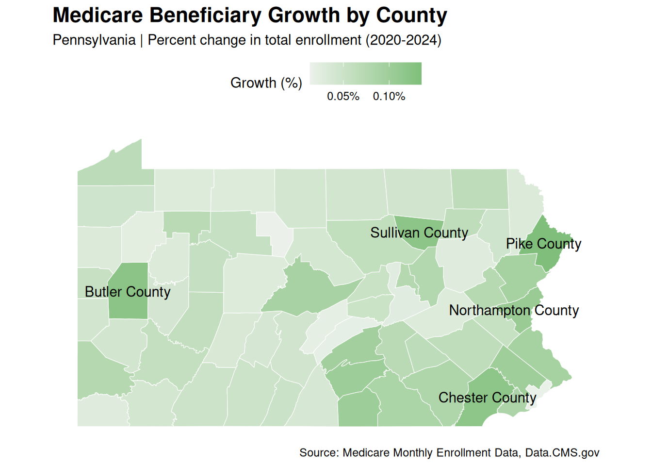
All data are public and sourced from Data.CMS.gov
Disclaimer: The findings, interpretation, and conclusions expressed herein are those of the authors and do not necessarily reflect the views of Centers for Medicare and Medicaid Services. All errors remain our own.
Footnotes
Note that some of the filtering and subseting occurred in the API call. Keeping these steps included here allow for transparency as well as the ability reproduce with the full dataset↩︎