---
title: "Quarto Demo for DSAC/Eng CoP"
subtitle: "`r paste('Medicare Growth in', params$state)`"
date: now
date-format: "MMMM D, YYYY"
language:
title-block-published: "Last Updated"
execute:
echo: false
warning: false
format:
html:
toc: true
theme: cosmo
css: dsac-theme.css
code-tools: true
code_fold: true
params:
state: "Pennsylvania"
start_year: 2020
end_year: 2024
---
```{r}
#| label: interactive-dev
# For interactive development only
if (interactive() && !exists("params")) {
params <- list(
state = "Pennsylvania",
start_year = 2020,
end_year = 2024
)
}
```
```{r}
#| label: dependencies
#| output: false
#| warnings: false
#| echo: false
library(tidyverse)
library(httr2)
library(sf)
library(tigris)
library(scales)
library(gt)
options(tigris_use_cache = TRUE)
```
::: {.callout-tip}
## Souped up version!
The differences here from the base version are that:
1. additional yaml matter (e.g. dynamic date, dynamic subtitle, default turning off code rendering)
1. code can now be viewed by the reader by clicking a link in the upper right hand corner
1. Table of Contents added for easier navigation
1. custom css formatting applied from an external css file in the repo
1. `params` added to yaml that allow us to use those repeated parameters throughout the report and allows us to use this as parameterized report template, i.e. we can render this report for every state
:::
::: {.callout-warning}
This demo report relies on R, but you can use R, Python, Julia, and Observable.
This demo report renders a document, but Quarto has a number of output options including documents, presentations, dahboards, websites, books.
:::
# BACKGROUND
This is an **important** annual report where we compare growth in beneficiaries at the county level in `r params$state`. Public data on [monthly Medicare enrollments](https://data.cms.gov/summary-statistics-on-beneficiary-enrollment/medicare-and-medicaid-reports/medicare-monthly-enrollment) were pulled from Data.CMS.gov using the [API](https://data.cms.gov/summary-statistics-on-beneficiary-enrollment/medicare-and-medicaid-reports/medicare-monthly-enrollment/api-docs).
::: {.callout-tip}
We can show important code even if most are not shown by default, using `echo: true` in this code chunk. This chunk also includes `code-fold: true` to that it is accessible, but tucked away.
:::
```{r}
#| label: fetch_api
#| echo: true
#| code-fold: true
# function to fetch data from data.cms.gov
fetch_data <- function(state, year, dataset_uuid,
                       baseurl = "https://data.cms.gov/data-api/v1") {

  endpoint <- stringr::str_glue("{baseurl}/dataset/{dataset_uuid}/data")

  cols <- paste(
    c("BENE_STATE_DESC", "BENE_STATE_ABRVTN", "BENE_COUNTY_DESC",
      "BENE_FIPS_CD", "BENE_GEO_LVL", "YEAR", "MONTH", "TOT_BENES"),
    collapse = ","
  )

  httr2::request(endpoint) |>
    httr2::req_url_query(
      `filter[BENE_STATE_ABRVTN]` = state,
      `filter[YEAR]` = year,
      `filter[BENE_GEO_LVL]` = "County",
      `filter[MONTH]` = "Year",
      column = cols
    ) |>
    httr2::req_throttle(rate = 2) |>  #max requests/sec
    httr2::req_retry(max_tries = 3) |>
    httr2::req_perform() |>
    httr2::resp_body_json()

}
```
```{r}
#| label: api_params
#parameters & global variables
#dataset type indentifier
dataset_uuid <- "d7fabe1e-d19b-4333-9eff-e80e0643f2fd"
#states of interest
states <- c("PA", "NY", "CA", "TX", "FL")
#years of interest
years <- c("2020", "2024")
#form expanded tibble for params to pull
api_params <- expand_grid(
state = states,
year = years,
dataset_uuid = dataset_uuid
)
#local dataset path
path_data <- "Data/medicare-monthly-enrollment_2025Oct_subset.csv"
```
```{r}
#| label: data_access
#run API if file doesn't already exist
if (!file.exists(path_data)) {
#API pull
df_pull <- api_params |>
pmap(
possibly(fetch_data, otherwise = NULL),
.progress = TRUE
) |>
bind_rows()
#create data folder if it doesn't exist
dir.create(dirname(path_data), showWarnings = FALSE)
#store data locally
write_csv(df_pull, path_data, na = "")
}
```
```{r}
#| label: read_data
#read in data
df <- read_csv(
path_data,
col_types = c(year = "i", tot_benes = "i", .default = "c"),
na = c("", "NA", "*"),
name_repair = tolower
)
```
The Medicare beneficiary dataset for this analysis pulled down just a subset of the rows and columns of the full data - `r scales::label_comma()(nrow(df))` rows and `r ncol(df)` columns. The analysis is focusing in on only the total beneficiary counts (`tot_benes`) in `r params$state` counties in `r params$start_year` to `r params$end_year`.
## Initial Munge
Once the data were loaded, we clean them for ease of use and to calculate the growth rate over this period in time. The following munging steps were performed^[Note that some of the filtering and subseting occurred in the API call. Keeping these steps included here allow for transparency as well as the ability reproduce with the full dataset]:
- renamed columns for ease of use
- filtered down the data to the particular state and focal years
- subset the columns to only those that were needed for analysis
```{r}
#| label: initial_munge
#subset dataset
df_lim <- df |>
rename(
state = bene_state_desc,
state_abbr = bene_state_abrvtn,
county = bene_county_desc,
county_fips = bene_fips_cd
) |>
filter(
state == params$state,
month == "Year",
bene_geo_lvl == "County",
year %in% c(params$start_year, params$end_year)
)
#limit to cols of interest
df_lim <- df_lim |>
select(year, state, state_abbr, county, county_fips, tot_benes)
```
## Access Spatial Data
We also brought in spatial data to map the growth rates across the state, leveraging the [`tigris` package](https://github.com/walkerke/tigris).
```{r}
#| label: spatial
#| include: false
# Download county boundaries for your state
state_counties <- counties(
state = unique(df_lim$state_abbr),
cb = TRUE,
year = max(df_lim$year)
)
# Convert to sf object if needed
state_counties_sf <- st_as_sf(state_counties)
# Ensure FIPS codes match data format
state_counties_sf <- state_counties_sf |>
mutate(county_fips = GEOID)
```
# IMPORTANT ANALYSIS SECTION
Time to do some calculations!
## Calculate Growth Rate
We calcualted growth rates to identify the counties with the largest growth during this period.
::: {.callout-note collapse="true"}
## Growth Rate Calculation
`growth rate = (end value / start value) - 1 `
:::
```{r}
#| label: pivot
#reshape
df_gr <- df_lim |>
mutate(pd = ifelse(year == max(year), "end", "start")) |>
select(-year) |>
pivot_wider(
names_from = pd,
values_from = tot_benes
)
df_gr <- df_gr |>
mutate(
gr_pct = (end - start) / start,
gr_abs = end - start
)
```
## Join Data
Before we were able to visualize it, we needed to join the spatial data with the enrollment data using the county FIPS codes.
::: {.callout-tip}
This is another example of showing an important code even if most are not shown by default, using `echo: true` in this code chunk.
:::
```{r}
#| label: merge
#| echo: true
df_viz <- left_join(state_counties_sf, df_gr, by = "county_fips")
```
# VIZ
Okay, time for the fun stuff - data viz!
## Top Counties
Here is a table (@tbl-growth-rates) of `r params$state`'s largest counties in terms of growth rate over this period.
```{r}
#| label: tbl-growth-rates
#| tbl-cap: Counties with the largest growth rates
#| output: true
df_gr |>
slice_max(order_by = gr_pct, n = 5) |>
select(county, start, end, gr_pct) |>
gt() |>
fmt_number(
columns = c(start, end),
decimals = 0
) |>
fmt_percent(
columns = gr_pct,
decimals = 1
) |>
cols_label(
county = "County",
start = 2020,
end = 2024,
gr_pct = "Growth Rate"
)
```
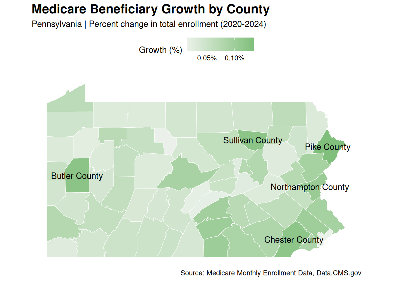
## State Map
We can visualize all `r params$state`'s county growth rate data for comparison in a map (@fig-growth-rate).
```{r}
#| label: fig-growth-rate
#| fig-cap: County Growth Rates
#| output: true
#| warnings: false
subt <- str_glue(
"{params$state} | Percent change in total enrollment ",
"({params$start_year}-{params$end_year})"
)
df_viz |>
ggplot() +
geom_sf(aes(fill = gr_pct), color = "white", size = 0.2) +
geom_sf_text(
data = df_viz |> slice_max(order_by = gr_pct, n = 5),
aes(label = county), na.rm = TRUE,
) +
scale_fill_gradient2(
low = "#af8dc3",
mid = "#f7f7f7",
high = "#7fbf7b",
midpoint = 0,
name = "Growth (%)",
labels = percent_format(scale = 1)
) +
labs(
x = NULL, y = NULL,
title = "Medicare Beneficiary Growth by County",
subtitle = subt,
caption = "Source: Medicare Monthly Enrollment Data, Data.CMS.gov"
) +
theme_minimal() +
theme(
plot.title = element_text(face = "bold", size = 16),
legend.position = "top",
axis.text = element_blank(),
axis.ticks = element_blank(),
panel.grid = element_blank()
)
```
# PARAMETERIZE
::: {.callout-note}
This qmd file now includes parameters (`params`) in the yaml. The parameters can be used through the documents (e.g. used to filter by state and years, dynamic text for titles/references).
The parameters can be changed manually and re-render, but we can pass the parameters through the render command in the terminal, a makefile, or another script to run this over multiple states or year and outputs.
From another Quarto or R script you could write the following code.
```
library(quarto)
library(purrr)

walk(
  c("Texas", "California", "New York"),
  ~ quarto_render(
    input = "demo_fancy.qmd",
    output_format = "pdf"
    execute_params = list(
      state = .x,
      start_year = 2020,
      end_year = 2024
    ),
    output_file = paste0("medicare_growth_", .x, ".pdf")
  )
)
```
:::
---
*All data are public and sourced from [Data.CMS.gov](https://data.cms.gov)*
*Disclaimer: The findings, interpretation, and conclusions expressed herein are those of the authors and do not necessarily reflect the views of Centers for Medicare and Medicaid Services. All errors remain our own.*